Chi-Square Test of Independence

[ | ]

Is there a relationship between whether or not a defendant has a gang charge (`gang`) and their race (`race`)?

Here, we’ll be working from the Defendants2025 data set, to examine the relationship between if a defendant has a gang charge (gang: measured as a categorical/nominal “yes” or “no”) and the defendant’s race (race: a nominal variable for each racial category).

What is the Chi Square Test of Independence?

The Chi Square test (\(X^2\)) examines the association or relationship between two nominal/ordinal variables to see if the relationship reflects a true relationship that we could expect to find in the population. The test also tells us whether or not a category (attribute) of one variable varies by categories of another variable.

The test is called the test of independence because it really tests the absence of association between (independence of) two variables.

Load the Necessary Stuff

library(MASS)
library(psych)
library(vannstats)

Reading in the Data

data1 <- Defendants2025

Assumptions and Diagnostics for Chi Square

The assumptions for the Chi Square are…

Independence of Observations
Normality

1. Independence of Observations (Examine Data Collection Strategy)

Cases (observations) are not related or dependent upon each other. Case can’t have more than one attribute. No ties between observations. Examine data collection strategy to see if there are linkages between observations.
- Given that the Defendants2025 data have been randomly-sampled, we have met the assumption of independence of observations.

2. Normality (Examine Expected Frequencies Crosstab/Contingency Table)

Distributions must be relatively normal.The normality assumption is met if no more than 20 percent of the cells in our Expected Frequencies crosstab have fewer than 5 cases. Therefore, if (\(E \lt 5\)) for more than 20 percent of the cells in the Expected Frequencies table, the assumption of normality is violated. If the assmuption of normality is violated, the researcher can employ Yates’ Continuity Correction, which conservatively adjusts the numerator for small sample sizes. To employ this correction in R, simply change the option to correct = TRUE.

In the vannstats package, I have included the tab function which returns the crosstabs of observed and expected frequencies. To check if you’ve met the assumption of normality (e.g. fewer than 20% of cells in the crosstab of expected frequencies falls below \(n=5\)), you use the following:

tab(data1, gang, race)

## $`Observed Frequencies`
##          race: asian black latine other white Total
## gang: no          68   315    673    34   344  1434
## yes                2   120    144     0    38   304
## Total             70   435    817    34   382  1738
## 
## $`Expected Frequencies`
##          race: asian     black   latine     other     white Total
## gang: no    57.75604 358.91254 674.0955 28.052934 315.18297  1434
## yes         12.24396  76.08746 142.9045  5.947066  66.81703   304
## Total       70.00000 435.00000 817.0000 34.000000 382.00000  1738

We see here that we have met the assumption of normality: less than 20% of cells in the 2x2 Expected Frequency crosstab have fewer than 5 expected counts. Actually, no cell has fewer than 5.

The Chi Square Test Calculation

The calculation for the Chi Square is:

\(X^2 = \sum \frac{(f_o - f_e)^2}{f_e}\) or \(X^2 = \sum \frac{(f_{o_i} - f_{e_i})^2}{f_{e_i}}\)

where…

\(f_o\) (or \(f_{o_i}\)) is the observed frequency for that cell (the \(i^{th}\)cell)
\(f_e\) (or \(f_{e_i}\)) is the expected frequency for that cell (the \(i^{th}\)cell)
- \(f_e\) (or \(f_{e_i}\)) for each cell is calculated by the following:
  - \(f_e\) (or \(f_{e_i}\)) \(= \frac{(r_{total_i})(c_{total_i})}{total}\) \(= \frac{(n_{row_i})(n_{column_i})}{N}\)

In addition, the degrees of freedom (\(df\)) for the test is…
* \(df = (r-1)(c-1)\)

where…

\(r\) is the number of rows in a crosstabulation
\(c\) is the number of columns in a crosstabulation

Running the Chi Square Test

For Chi Square, within the chi.sq function, the dependent variable is listed first and the independent variable is listed second.

#chisq.test(data1$gang, data1$race, correct=FALSE)
chi <- chi.sq(data1, gang, race)
summary(chi)

## Call:
## chi.sq(df = data1, var1 = gang, var2 = race)
## 
## Pearson's Chi-squared test: 
## 
##      χ² Critical χ² df   p-value    
##  63.385       9.488  4 5.632e-13 ***
## ---
## Signif. codes:  0 '***' 0.001 '**' 0.01 '*' 0.05 '.' 0.1 ' ' 1

In the output above, we see the \(X^2\)-obtained value (63.385), the degrees of freedom (4), and the p-value (5.632e-13, or .0000000000005632, which is less than our set alpha level of .05).

To interpret the findings, we report the following information:

The test used
If you reject or fail to reject the null hypothesis
The variables used in the analysis
The degrees of freedom, calculated value of the test (\(X^2_{obtained}\)), and \(p-value\)
- \(X^2(df) = X^2_{obtained}\), \(p-value\)

“Using the Chi Square test of independence (\(X^2\)), I reject/fail to reject the null hypothesis that there is no association between variable one and variable 2, in the population, \(X^2(?) = ?, p ? .05\)”

“Using the Chi Square test of independence (\(X^2\)), I reject the null hypothesis that there is no association between the whether or not a defendant gets a gun charge and their race, in the population, \(X^2(4) = 63.385, p \lt .05\)”

Yates’ Continuity Correction for the Chi Square Test

The calculation for Yates’ Chi Square is:

\(X^{2}_{Yates'} = \sum \frac{(|f_o - f_e| - 0.5)^2}{f_e}\) or
\(X^{2}_{Yates'} = \sum \frac{(|f_{o_i} - f_{e_i}| - 0.5)^2}{f_{e_i}}\)

To employ Yates’ Continuity Correction, when we have violated the assumption of normality, simply update the chi.sq option to correct = TRUE, like this:

chi <- chi.sq(data1, gang, race, correct=TRUE)
summary(chi)

Post-Hoc Significance Test

After finding a significant result in your omnibus/overall chi square test, to identify where the differences lie, you can run a post-hoc significance test.

We can see where the significantly different comparisons (between observed and expected) are both in a table and a visual (plot) format, using Bonferroni’s adjusted p-values, which can be called from the chi.sq function, using the following:

chi <- chi.sq(data1, gang, race, post = T, plot = T)

summary(chi)

## Call:
## chi.sq(df = data1, var1 = gang, var2 = race, post = T, plot = T)
## 
## Pearson's Chi-squared test: 
## 
##      χ² Critical χ² df   p-value    
##  63.385       9.488  4 5.632e-13 ***
## ---
## Signif. codes:  0 '***' 0.001 '**' 0.01 '*' 0.05 '.' 0.1 ' ' 1
## 
## 
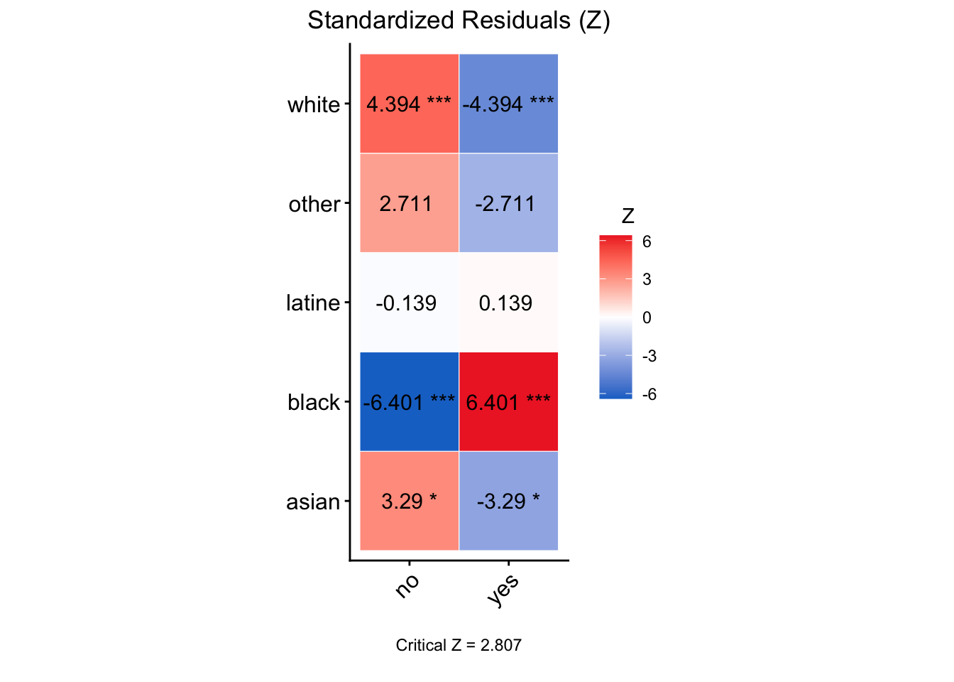
## Post-Hoc Test w/ Bonferroni Adjustment:
## Comparing: race-gang 
## 
##            Standardized Residual (Z)   p-value    
## asian-no                      3.2899 0.0100219 *  
## asian-yes                    -3.2899 0.0100219 *  
## black-no                     -6.4008 1.546e-09 ***
## black-yes                     6.4008 1.546e-09 ***
## latine-no                    -0.1386 1.0000000    
## latine-yes                    0.1386 1.0000000    
## other-no                      2.7114 0.0670021 .  
## other-yes                    -2.7114 0.0670021 .  
## white-no                      4.3939 0.0001113 ***
## white-yes                    -4.3939 0.0001113 ***
## ---
## Signif. codes:  0 '***' 0.001 '**' 0.01 '*' 0.05 '.' 0.1 ' ' 1

As seen above:

Here, we see that asian defendants are more likely to be not given a gang charge (and less likely to be given a gang charge), that black defendants are more likely to be given a gang charge (and less likely to not be given a gang charge), and that white defendants are more likely to not be given a gang charge (and less likely to be given a gang charge). These are areas where the disparity between being given (e.g. yes) and not being given (e.g. no), is significantly different.