Paired Samples (Repeated Measures) t-Test
Are there mean differences in the risk score of our defendants at
time one (risk_score) compared to time two
(risk_score2)?
Here, we’ll be working from the Defendants2025 data set, to
examine differences in the mean defendant’s risk score at time one
(risk_score: measured as an interval-ratio
variable) and time two (risk_score2: measured
as an interval-ratio variable).
What is the Paired Samples t-Test?
The paired samples t-test examines the differences in means between two measurement periods – the mean before (e.g. time one) and the mean after (e.g. time two) an event or manipulation.
Reading in the Data
Additionally, we need to incorporate a second variable (which we will
call risk_score2) with which to compare our
original risk score variable…
a <- c(7.48,4.03,4.19,5.13,8.48,7.68,1.77,2.48,3.70,2.98,2.40,2.91,6.78,6.60,2.43,6.18,3.98,5.99,5.66,6.56,1.50,4.40,2.42,8.21,4.73,1.92,4.04,5.41,3.76,9.36,5.35,6.34,8.97,3.71,3.78,2.10,2.96,1.96,9.07,9.27,4.73,0.95,8.14,6.87,2.42,8.12,5.52,1.26,5.00,9.37,7.28,1.83,3.69,1.09,5.22,7.22,1.58,2.24,2.03,2.95,3.41,8.46,8.53,3.64,6.66,3.94,1.74,5.27,6.47,5.16,1.51,7.93,3.40,5.94,6.59,6.90,5.81,0.82,2.46,1.67,4.11,6.96,4.32,4.71,1.11,5.39,6.47,1.61,8.64,7.50,3.67,6.97,5.55,4.30,8.75,2.01,2.63,4.58,5.73,7.48,4.30,2.92,6.34,8.83,3.88,7.28,5.91,2.26,4.80,8.27,8.47,1.65,7.29,2.33,8.49,0.72,8.61,2.93,2.48,6.86,1.40,8.76,9.34,6.07,3.31,5.76,5.48,6.35,5.85,4.40,6.85,4.32,7.62,7.40,2.36,1.91,2.08,0.70,2.66,5.10,0.90,8.34,6.91,6.20,5.15,2.25,4.42,3.79,4.33,5.59,2.63,8.44,5.26,6.31,5.09,1.44,2.16,8.33,6.72,4.74,4.48,6.61,5.73,4.57,5.78,7.03,9.17,6.97,1.37,2.87,1.83,2.51,9.18,4.05,6.14,1.60,7.34,1.95,2.07,4.35,6.54,6.10,7.34,7.15,6.22,7.68,1.91,5.94,5.90,5.60,6.09,6.95,2.41,6.50,6.60,1.70,6.61,1.24,3.82,8.93,3.81,3.96,2.33,8.35,4.01,1.59,5.96,9.06,5.01,6.94,8.40,4.10,2.36,7.85,5.16,4.18,2.77,4.41,9.25,5.67,1.59,2.44,0.97,3.17,6.50,6.52,1.43,1.26,3.69,7.29,5.80,8.87,9.00,1.17,2.13,5.85,6.58,5.11,9.00,4.71,4.32,3.19,8.44,5.13,5.35,4.17,2.92,6.80,6.09,4.04,2.97,5.04,1.48,9.46,2.82,5.22,1.43,6.01,2.79,6.71,2.85,2.99,8.66,7.02,8.27,2.06,6.92,7.44,5.04,1.42,8.49,4.22,2.66,1.32,1.50,7.59,1.75,8.41,3.97,5.11,0.81,9.38,5.85,4.16,1.71,5.00,1.98,9.39,4.94,2.92,4.79,1.35,5.79,7.66,0.96,8.70,2.16,1.33,3.89,0.74,2.37,1.49,2.28,6.90,4.27,8.43,3.77,3.68,7.39,5.14,4.77,6.89,2.21,5.07,5.00,5.12,5.58,1.95,2.26,2.50,4.86,3.30,2.58,1.00,4.77,8.76,2.66,6.91,0.84,3.93,4.33,7.60,5.77,1.93,2.22,6.57,2.18,5.47,5.03,5.14,8.72,5.86,2.07,5.36,1.96,4.14,4.71,8.65,6.61,3.35,4.68,4.68,4.54,3.54,3.67,6.85,8.18,1.40,6.80,8.67,4.14,4.56,0.90,3.16,4.77,5.97,2.84,5.16,7.26,4.66,8.66,1.53,9.42,3.66,9.45,5.50,1.40,1.71,8.20,8.87,6.40,1.83,4.46,5.74,6.17,6.42,2.81,5.04,6.53,3.38,8.93,4.99,2.03,3.88,5.80,5.67,9.21,6.46,6.79,2.97,1.40,1.82,3.91,7.11,6.36,3.32,1.60,0.96,6.58,7.87,9.08,1.98,5.65,1.09,4.75,1.59,3.20,5.66,5.15,7.85,1.24,7.53,5.36,7.83,1.33,8.13,8.71,5.50,1.01,8.24,9.15,1.91,0.79,0.84,5.07,3.99,9.38,0.82,7.54,8.00,4.08,4.37,7.12,6.86,7.56,8.54,8.83,3.05,9.09,5.11,2.70,5.94,2.49,1.37,8.33,1.86,3.51,3.51,2.01,8.01,7.39,7.27,1.11,2.95,6.53,5.02,9.44,9.28,8.71,7.02,6.19,3.25,2.79,2.35,2.48,7.71,5.98,8.73,2.39,8.40,3.66,2.82,7.32,5.20,4.20,5.89,3.70,1.77,2.46,6.06,7.99,5.32,1.67,3.68,6.22,9.23,9.22,3.23,3.59,4.53,7.18,5.63,5.55,4.50,8.64,6.32,7.81,6.46,5.14,4.39,7.99,6.49,9.38,7.07,5.69,8.32,7.68,8.79,3.97,1.91,0.90,8.53,3.02,0.95,5.87,4.47,4.05,6.77,2.41,2.30,9.23,2.18,5.40,5.62,5.74,2.43,8.69,0.88,5.80,5.73,8.55,8.35,5.73,5.46,7.88,7.47,6.34,3.57,7.05,7.33,5.27,0.81,5.13,3.73,7.41,3.26,2.01,7.12,4.06,6.45,3.44,9.31,5.16,6.66,2.07,2.51,3.77,7.52,2.95,7.57,0.87,1.13,7.13,1.90,9.01,9.26,7.68,5.61,1.87,1.78,1.14,3.17,9.41,5.18,6.25,3.14,4.94,1.87,3.60,6.79,1.63,7.91,8.91,8.82,3.46,6.93,4.06,4.42,1.39,2.31,1.56,9.41,0.69,1.37,1.17,2.33,2.07,4.34,5.71,2.04,1.76,8.36,8.74,2.68,1.13,8.30,1.20,2.46,9.06,1.79,5.74,8.97,6.84,1.69,8.74,9.38,2.98,8.10,7.14,9.31,5.75,8.59,4.21,7.46,6.43,1.89,0.67,6.12,3.48,1.96,9.03,6.68,3.33,8.39,0.68,3.49,4.87,1.12,8.72,5.34,2.31,4.30,8.98,3.04,7.32,7.74,2.69,2.89,1.46,2.95,4.79,6.24,6.36,2.66,0.74,5.29,3.35,5.43,1.34,4.62,1.19,2.27,4.73,7.07,2.81,2.89,1.96,1.77,3.61,3.41,6.62,3.42,6.00,4.95,2.73,7.08,5.35,2.24,5.96,1.21,6.36,5.79,1.50,2.05,3.01,6.28,4.94,7.11,7.24,3.23,1.58,3.90,6.42,8.87,8.70,3.96,1.28,4.63,6.11,4.42,1.77,6.82,3.34,3.15,9.31,7.89,1.32,3.91,1.54,5.25,3.00,2.33,2.01,7.41,0.98,5.61,1.20,2.30,7.89,0.98,8.59,6.82,7.03,3.73,7.64,6.73,2.31,1.95,1.54,9.05,3.51,4.30,5.96,6.13,3.46,7.50,8.06,9.11,2.56,3.42,9.17,4.16,6.98,7.54,4.75,6.17,5.83,3.54,8.86,7.02,8.63,7.09,6.13,0.67,4.73,7.68,2.55,1.06,3.13,8.30,2.96,4.87,7.06,4.85,8.87,5.64,3.68,4.37,8.19,8.69,2.65,4.58,3.41,2.55,8.69,8.14,7.76,1.03,2.45,5.40,4.74,8.72,2.81,4.46,9.22,8.30)
b <- c(2.80,0.93,6.16,1.98,8.25,3.58,1.95,6.93,9.22,4.58,7.78,3.65,8.04,1.78,8.02,6.78,4.93,5.64,1.44,1.74,6.74,1.67,3.22,3.65,2.74,2.47,3.58,2.55,2.23,6.56,5.19,5.49,6.44,9.09,1.75,0.78,4.78,2.42,6.73,7.20,4.27,5.84,3.97,6.23,3.43,5.60,0.94,1.85,6.65,8.50,2.09,4.49,4.34,8.89,1.98,5.92,7.40,6.80,7.18,3.38,1.74,5.28,0.74,9.17,7.05,3.02,6.41,6.68,2.03,5.81,5.73,4.88,3.37,8.98,1.54,4.04,8.94,7.58,7.12,7.33,2.94,4.30,6.86,4.26,6.71,3.22,0.95,7.25,4.72,2.17,8.70,5.19,1.08,6.01,6.71,8.96,4.04,2.38,2.48,5.55,1.48,2.19,3.04,4.01,8.92,3.40,5.74,6.22,3.05,2.89,1.56,2.11,7.06,4.65,5.65,8.05,8.79,1.06,9.18,9.44,1.05,2.34,3.14,4.68,3.42,3.59,2.56,2.96,0.82,2.41,7.38,4.67,9.42,5.80,7.66,4.54,3.28,1.25,8.19,5.00,1.05,5.52,0.77,5.32,4.98,5.57,4.83,1.39,6.83,2.86,2.89,3.27,2.12,5.07,6.86,3.33,3.92,6.73,2.01,3.83,7.44,1.58,3.85,3.48,3.08,6.36,8.90,5.25,2.13,4.00,9.11,1.98,6.15,3.61,3.58,9.17,5.57,9.19,0.87,4.65,3.92,1.31,3.80,5.99,5.30,5.14,2.29,3.19,1.43,8.52,1.65,6.80,3.06,4.43,8.81,0.90,6.83,8.22,4.73,8.23,8.43,5.28,0.81,8.65,9.14,0.68,6.38,2.08,5.37,8.55,9.16,5.93,9.04,1.41,6.82,7.92,7.32,7.32,6.70,1.75,8.08,4.65,5.55,8.08,6.61,2.54,6.72,3.30,3.38,4.46,5.58,8.25,6.96,1.64,3.35,6.51,1.21,8.42,6.09,0.91,4.12,7.10,6.29,7.99,9.10,1.84,8.85,5.24,8.11,9.37,5.07,4.95,5.60,7.77,3.94,6.83,7.76,7.54,7.54,8.97,8.58,5.36,6.37,4.26,4.05,8.35,8.46,2.06,2.53,9.09,8.16,6.53,8.29,5.41,4.23,9.26,5.06,5.01,4.40,2.46,1.06,8.92,0.97,2.51,8.50,8.09,5.24,8.19,5.33,6.92,8.84,1.03,9.43,8.29,0.79,4.79,3.05,7.44,7.57,9.08,5.62,7.85,4.14,8.25,6.64,0.88,2.50,5.64,1.74,3.35,1.47,8.20,1.86,6.98,1.37,8.12,8.05,3.41,1.47,0.88,0.79,1.04,3.76,0.70,9.22,7.97,6.18,3.18,7.15,1.23,6.15,6.24,8.41,4.82,1.71,6.10,4.28,0.70,7.92,4.31,3.54,6.89,9.22,6.03,4.02,5.32,6.39,4.40,5.50,4.94,4.04,5.08,6.09,7.20,3.09,9.27,2.02,3.00,5.82,4.94,5.43,3.92,2.28,7.62,0.76,3.14,3.98,5.34,7.62,7.21,5.61,4.52,9.19,5.97,5.81,3.43,5.00,8.50,4.02,8.40,9.15,8.15,1.24,0.98,1.29,8.09,5.03,2.46,9.39,4.61,7.99,8.49,6.42,1.38,8.28,6.12,1.67,0.97,6.43,4.45,1.77,5.59,6.68,7.05,7.18,6.38,0.89,6.50,8.91,7.66,3.26,8.42,4.53,8.57,6.63,3.18,1.00,5.43,1.87,5.27,5.47,8.11,6.08,3.42,3.73,2.42,8.54,8.60,6.79,2.01,8.58,2.23,3.48,5.71,1.72,4.27,8.99,2.98,7.68,1.37,4.60,4.23,7.37,1.32,2.94,3.13,7.97,3.63,4.34,6.98,4.02,2.82,7.23,5.68,2.42,8.28,2.34,3.35,9.06,2.74,3.49,1.82,7.10,9.20,8.04,8.78,3.69,6.22,6.99,0.77,3.35,5.34,6.88,7.60,5.17,6.68,7.93,6.72,1.57,1.27,6.19,5.35,5.08,4.23,6.49,6.43,3.89,7.40,5.36,1.38,1.36,1.39,3.71,7.51,4.94,1.79,4.44,4.34,5.09,5.11,6.17,2.26,6.09,1.33,8.90,5.86,4.01,1.26,8.98,1.88,7.47,0.93,2.79,8.36,3.45,7.37,6.31,8.03,8.33,1.92,9.39,2.35,4.28,2.71,3.22,5.53,0.91,4.89,2.09,2.41,8.72,4.95,2.77,2.18,2.53,8.42,7.32,5.23,8.16,9.45,1.52,1.73,1.54,4.56,8.49,1.30,7.90,7.20,6.17,8.30,8.38,4.55,2.18,1.34,7.61,2.10,3.20,4.83,4.11,8.59,7.96,1.57,6.21,7.18,4.90,6.83,6.15,2.12,8.23,5.06,2.62,7.43,1.02,3.16,4.01,2.58,5.01,2.70,1.46,0.99,5.43,7.22,7.03,0.86,9.41,0.90,3.35,5.21,7.55,5.51,5.92,7.08,7.43,5.21,1.56,4.47,2.79,4.66,8.14,7.70,6.97,5.12,1.76,7.32,1.37,8.99,3.44,9.11,2.37,5.29,6.65,5.19,4.10,7.00,2.58,4.78,2.28,4.75,9.40,6.80,2.57,6.80,8.43,6.21,9.37,3.50,9.38,7.03,4.27,3.59,6.90,4.92,1.51,6.73,8.85,5.04,8.36,7.81,3.18,5.23,0.99,3.68,6.32,8.43,9.21,8.52,1.99,3.12,3.28,2.82,6.32,8.48,4.98,1.76,1.10,0.72,0.72,2.03,4.00,4.33,3.86,6.30,5.58,8.62,4.05,8.66,9.41,8.46,6.29,8.43,1.90,7.40,7.45,8.61,0.88,3.78,2.25,2.51,9.45,9.31,7.79,3.44,5.40,1.22,1.55,4.26,3.73,6.22,8.14,8.11,7.15,4.88,3.78,7.27,7.29,8.62,2.33,4.67,9.35,5.27,2.58,7.81,5.12,3.34,9.27,0.80,8.78,8.93,7.70,9.21,2.07,3.33,8.48,8.83,0.71,4.32,8.63,5.85,1.30,5.03,7.07,3.44,6.52,1.93,5.69,3.40,2.11,3.80,4.41,9.06,4.45,4.33,6.63,4.61,4.36,4.03,7.00,2.00,3.88,1.06,5.29,7.34,7.63,7.00,7.04,3.32,3.61,1.20,6.00,6.01,6.64,9.35,0.95,3.79,3.09,2.14,7.10,5.97,3.55,5.25,8.53,6.87,3.42,7.17,3.26,1.40,3.01,4.64,2.79,2.13,5.83,2.30,8.26,5.14,2.83,6.63,7.55,8.56,1.79,3.55,6.97,4.92,9.03,4.11,2.97,1.71,1.83,2.84,8.74,4.13,2.90,9.38,3.93,4.32,1.51,6.54)
c <- c(1.09,1.50,2.08,0.94,2.13,9.06,4.67,6.13,7.42,9.39,6.27,6.22,5.29,1.26,9.16,7.93,2.83,9.26,8.24,1.51,8.19,6.46,6.13,1.78,8.18,1.54,6.34,5.92,6.81,8.49,6.73,2.60,7.91,9.06,7.27,1.65,4.23,6.20,4.84,1.96,1.44,5.68,6.71,4.00,1.34,4.95,2.67,4.97,1.97,1.52,4.59,3.82,9.35,5.70,9.20,6.47,6.87,7.76,4.23,3.07,9.01,4.73,1.44,2.19,0.92,6.12,2.58,8.54,7.21,5.40,6.71,2.72,4.90,4.65,6.07,4.47,5.89,1.23,4.19,5.06,6.90,1.62,6.68,7.56,4.61,5.25,9.37,0.90,6.46,6.10,4.17,3.99,6.01,2.55,5.05,2.06,5.05,2.84,1.27,2.25,7.03,1.95,7.03,8.33,8.75,1.01,1.96,0.78,5.14,1.92,8.15,3.75,2.45,5.52,2.98,2.39,6.59,6.75,9.39,1.81,8.93,7.00,3.48,6.71,3.00,5.35,1.59,8.82,4.73,1.21,3.19,6.39,7.49,6.41,9.31,4.54,1.38,2.46,7.54,7.92,2.34,7.12,6.13,7.67,6.44,5.14)
time2 <- c(a,b,c)

data1$risk_score2 <- time2
Assumptions and Diagnostics for the Paired Samples t-Test
The assumptions for a t-test are…
- Independence of Observations
- Normality
1. Independence of Observations (Examine Data Collection Strategy)
- Cases in our sample are independent of one another. Examine data
collection strategy to see if there are linkages between observations.
- Given that the
Defendants2025data have been randomly-sampled, we have met the assumption of independence of observations.
- Given that the
2. Normality (Examine Plots: Histogram, Q-Q Normality Plots, Box-and-Whiskers Plots)
- Distribution must be relatively normal. (If violated, use “unequal variances assumed” formula, otherwise, use “equal variances assumed”). In the past, you may have been instructed to use the Shapiro-Wilk test to assess normality. This is wrong. Unfortunately, tests such as these are overly-sensitive to trivial deviations from normality, and may result in you believing you must correct for normality by transforming your data. Please do not do this. The good thing is the t-test is super-robust – robust enough to provide results even in the presence of data that are not fully normally-distributed.
4a. Histogram
Plot the histogram for risk score at time one and the risk score at time two…
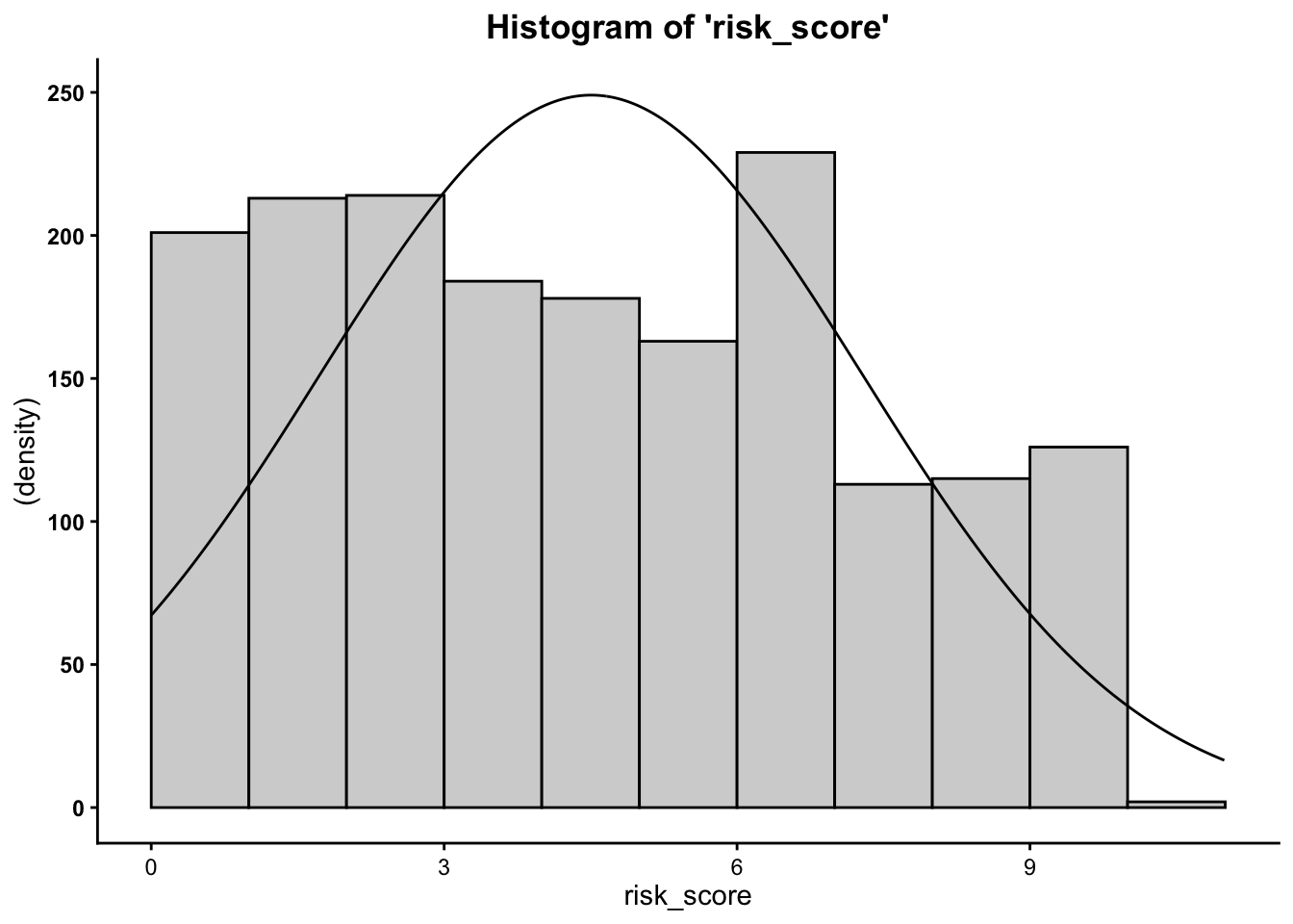
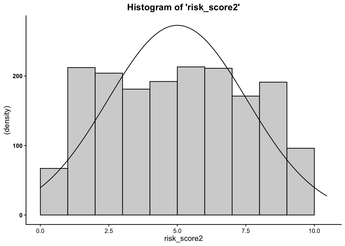
- We can see from the histograms that the
distribution of the outcome variable (
risk_scoreandrisk_score2) is relatively normal.
4b. Boxplots (Box-and-Whisker Plots)
Boxplots also provide a visual representation of the normality of a distribution. The boxplot has a box, a line through the box, two whiskers on either end of the box, and sometimes dots/points outside the whiskers. Below, we get a sense of what each part of the boxplot represents…
- Bottom (or left end) of the whisker represents the minimum score for that variable’s distribution
- Bottom (or left end) of the box represents the first quartile (the 25th percentile case)
- Middle line (or dot) inside the box represents the median, also known as the second quartile (the 50th percentile case)
- Top (or right end) of the box represents the third quartile (the 75th percentile case)
- Top (or right end) of the whisker represents the maximum score for that variable’s distribution
- Outside dots represent outliers - extreme high or extreme low values for that variable.
To tell if a variable is normally-distrubted using the box-and-whisker plot, generally, we want to see that there is some distance between the box and the end of the whiskers, that the box isn’t pushed too close to either whisker, that the median line (dot) is near the center of the box, and that there aren’t many outliers (dots) on the outside of the whiskers.
To plot a boxplot for risk score and
risk_score2, we do the following…
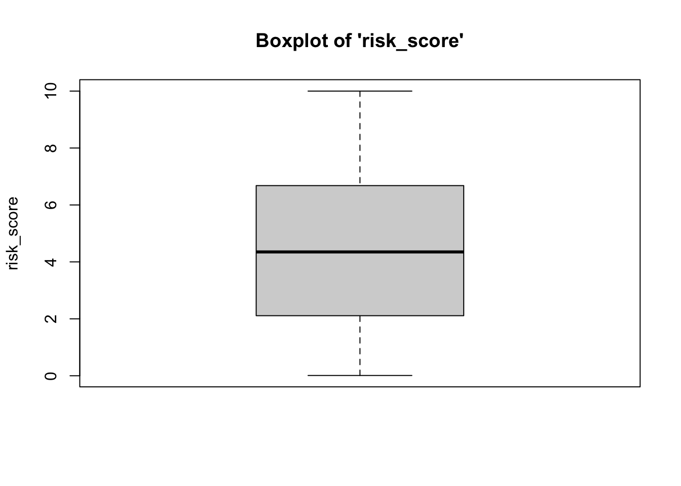
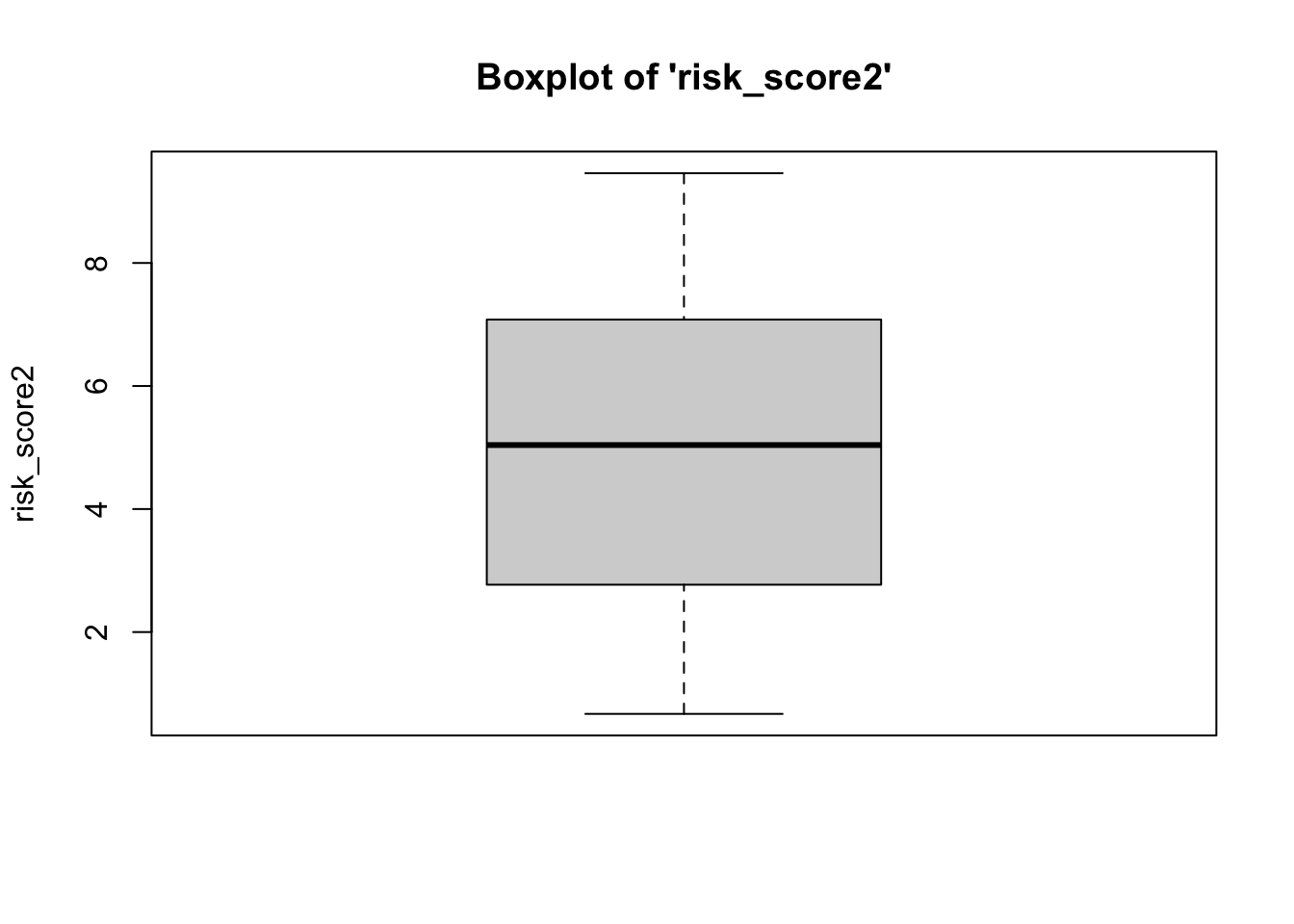
- We can see from the boxplots that the data are normally-distributed: The median falls in the center of the interquartile range and that interquartile range is centered between the whiskers. It is safe to assume that these data are close enough to normal, since they aren’t drastically different from normal, and therefore safe to proceed with the statistical test.
4c. Normal Q-Q (Quantile-Quantile) Plots
The quantile-quantile plot is a visual tool to help us figure out if the empirical distribution of our variable fits (or rather, comes from) a theoretical normal distribution.
We assess normality for risk score and
risk_score2, using the following
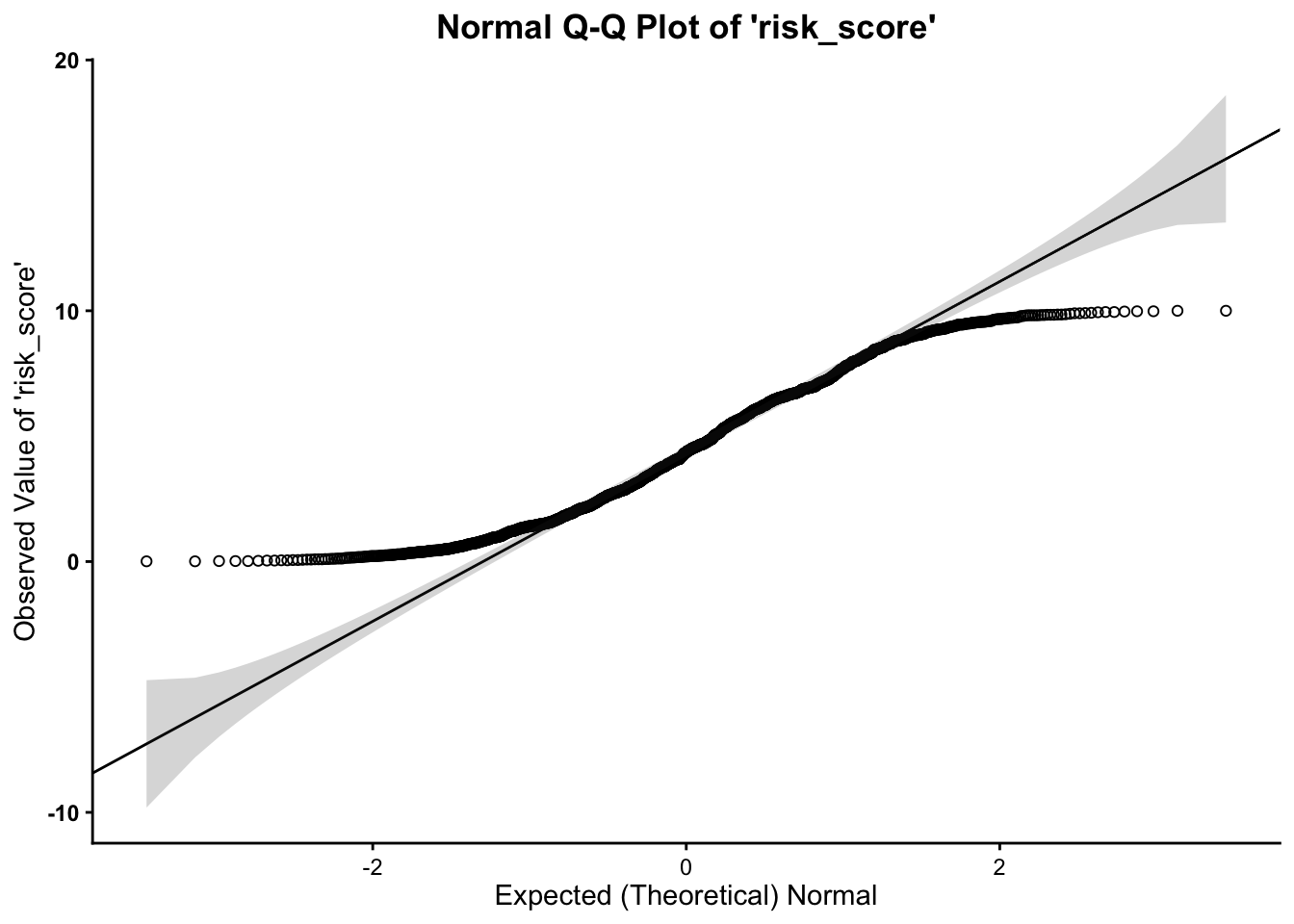
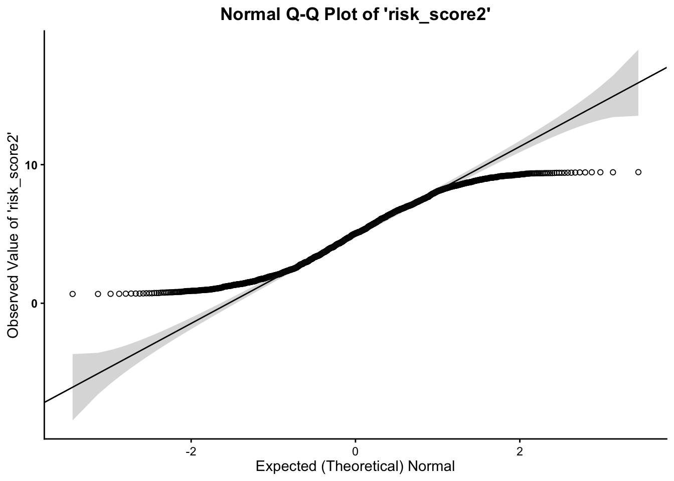
- We can see from the Q-Q plot that the
outcome variable (both
risk_scoreandrisk_score2) is normal, however, it is clear that the data tend to curl away from the normality line at the tails of the distribution. This indicates some deviation from normality. Therefore, it is safe to proceed with the statistical test.
- Across all three plots of the outcome
variable (both
risk_scoreandrisk_score2), the data do not seem to drastically deviate from normality. Therefore,we can assume normality.
The Paired Samples t-Test Calculation
The calculation for the t-Test is:
\(t = \frac{\bar{d}}{\frac{SD_d}{\sqrt{n}}}\)
where…
- \(\bar{d}\) is the mean of the
difference between time pairs
- \(SD_d\) is the standard deviation
for the difference between time pairs
- \(n\) is the sample size
(e.g. number of pairs)
In addition, the degrees of freedom (\(df\)) for the test is…
\(df = n - 1\)
Running the Paired Samples t-Test in R
To run the paired samples t-test in R, we use the traditional t.test function. But, in the
vannstats package, we can
use the ps.t.
Within the ps.t
function, the data frame is listed first, followed by the
(interval-ratio level) variable for the second time point, followed by
the (interval-ratio level) variable for the first time point.
If you meet the assumptions of the one sample t-test, you can
assume equal variances, which is assumed by default in
the function (using the call var.equal=TRUE). If you violate
this assumption, you must add the following call to the function: var.equal=FALSE.
## Call:
## ps.t(df = data1, t2 = risk_score2, t1 = risk_score)
##
## Paired Samples (Repeated Measures) t-test:
##
##       𝑡 Critical 𝑡   df   p-value
##  5.6197     1.9610 1737 2.224e-08 ***
## ---
## Signif. codes:  0 '***' 0.001 '**' 0.01 '*' 0.05 '.' 0.1 ' ' 1
##
## Group Means and Difference:
##  x̅: risk_score2   x̅: risk_score mean difference
##       5.0039241       4.5060242       0.4978999
In the output above, we see the t-obtained value 5.6197, or rather, \(\pm\) 5.6197), the degrees of freedom (1737), and the p-value (.00000002224, which is less than our set alpha level of .05).
To interpret the findings, we report the following information:
- The test used
- If you reject or fail to reject the null hypothesis
- The variables used in the analysis
- The degrees of freedom, calculated value of the test (\(t_{obtained}\)), and \(p-value\)
- \(t(df) = t_{obtained}\), \(p-value\)
“Using a one sample t-test, I reject/fail to reject the null hypothesis that there is no mean difference between time one and time two, in the population, \(t(?) = ?, p ? .05\)”
- “Using a paired samples t-test, I reject the null hypothesis that there is no difference between the mean risk scores for time one and time two, in the population, \(t(1737) = \pm 5.6197, p \lt .05\)”