One-Way Analysis of Variance
Are there mean differences in risk scores
(risk_score) by race of the defendant
(race)?
Here, we’ll be working from the Defendants2025 data set, to
examine mean differences in a defendant’s risk score
(risk_score: measured as an interval-ratio
variable) by race of the defendant (race:
across five racial categories).
What is the Analysis of Variance (ANOVA)?
The ANOVA test examines the differences in means between three or more groups, in effort to see if the differences reflect true differences that we could expect to find in the population. The resulting test calculates an F value.
Assumptions and Diagnostics for the One-Way ANOVA
The assumptions for an ANOVA are…
- Independence of Observations
- Equal Sample Sizes
- Homogeneity of Variance
- Normality
1. Independence of Observations (Examine Data Collection Strategy)
Groups are not related or dependent upon each other. Case can’t be in more than one group. No ties between observations. Examine data collection strategy to see if there are linkages between observations.
- Given that the
Defendants2025data have been randomly-sampled, we have met the assumption of independence of observations.
- Given that the
2. Equal Sample Sizes (Examine N for each group)
- The number of cases in each group should be relatively similar. Fortunately, ANOVA is relatively robust to small departures from equality. However, according to Keppel (1993) the equal sample sizes assumption matters because sample size affects group variances, and can therefore affect the homogeneity of variances assumption. The takeaway is: if you have unequal sample sizes but equal variances – no problem. The real issue is if you have both unequal sample sizes and unequal variances.
3. Homogeneity of Variance (Examine SD2 for each group)
- All groups have approximately equal variances (SD2). The distributions (or spread) for the groups are approximately equal. Keppel & Zedeck (1989) suggest that variance comparison should not exceed 10:1 ratio (or… alternatively, the SDs, when compared, should not exceed around a 3:1 ratio). In the past, you may have been instructed to use the Levene’s test to assess the degree of similarity in variances across groups. This is wrong. Unfortunately, tests such as these are overly-sensitive to trivial deviations from homogeneity of variance. It is a better practice to compare group variances/SDs based on the ratios listed above.
For both of the above assumptions, we can examine the univariate data table, broken out by group:
##
##  Descriptive statistics by group
## group: asian
##    vars  n mean   sd median trimmed  mad  min  max range skew kurtosis  se
## X1    1 70 3.14 2.54   2.36    2.77 1.44 0.04 9.22  9.18 1.22      0.3 0.3
## -----------------------------------------------------------
## group: black
##    vars   n mean   sd median trimmed  mad  min max range skew kurtosis   se
## X1    1 435 4.82 2.82   4.74     4.8 3.53 0.02  10  9.98 0.03    -1.22 0.14
## -----------------------------------------------------------
## group: latine
##    vars   n mean   sd median trimmed  mad  min max range skew kurtosis  se
## X1    1 817 4.82 2.81   4.96     4.8 3.31 0.01  10  9.99 0.01    -1.11 0.1
## -----------------------------------------------------------
## group: other
##    vars  n mean   sd median trimmed  mad  min  max range skew kurtosis   se
## X1    1 34 3.69 2.64   3.44    3.45 2.71 0.01 9.98  9.97 0.68    -0.22 0.45
## -----------------------------------------------------------
## group: white
##    vars   n mean   sd median trimmed mad  min  max range skew kurtosis   se
## X1 1 382 3.8 2.53 3.42 3.58 2.7 0.03 9.98 9.95 0.61 -0.36 0.13- Given that the group sizes are somewhat
different,
we have NOT met the assumption of equal sample sizes. However, given that the standard deviations for all five groups do not exceed a 3:1 ratio,we have met the assumption of homogeneity of variance.
4. Normality (Examine Plots: Histogram, Q-Q Normality Plots, Box-and-Whiskers Plots)
- Distribution must be relatively normal. (If violated, use “unequal variances assumed” formula, otherwise, use “equal variances assumed”). In the past, you may have been instructed to use the Shapiro-Wilk test to assess normality. This is wrong. Unfortunately, tests such as these are overly-sensitive to trivial deviations from normality, and may result in you believing you must correct for normality by transforming your data. Please do not do this. The good thing is ANOVA is robust enough to provide results even in the presence of data that are not fully normally-distributed.
4a. Histogram
Plot the histogram for risk_score (Y variable) broken
out by race (levels of the X variable)…
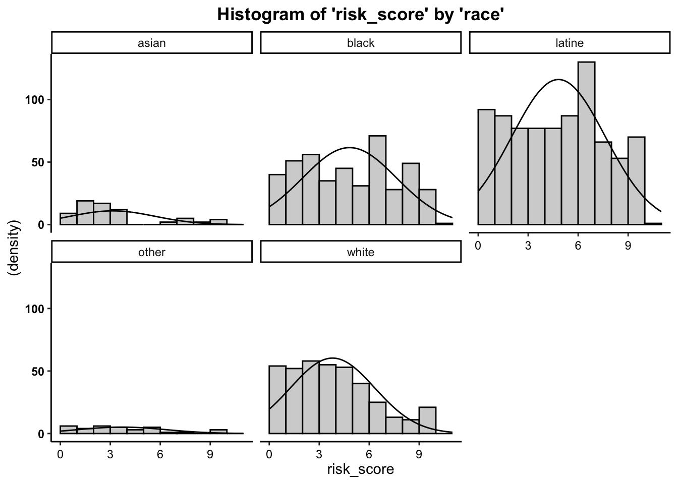
- We can see from the histograms that the
distributions of the outcome variable (
risk_score) by the predictor/grouping/independent variable (race), are relatively normal forblack,latine, andwhitedefendants. The small group sizes forasianandotherdefendants results in platykurtic distributions with longer right tails. Yet, overall, these data are close enough to normal.
4b. Boxplots (Box-and-Whisker Plots)
Boxplots also provide a visual representation of the normality of a distribution. The boxplot has a box, a line through the box, two whiskers on either end of the box, and sometimes dots/points outside the whiskers. Below, we get a sense of what each part of the boxplot represents…
- Bottom (or left end) of the whisker represents the minimum score for that variable’s distribution
- Bottom (or left end) of the box represents the first quartile (the 25th percentile case)
- Middle line (or dot) inside the box represents the median, also known as the second quartile (the 50th percentile case)
- Top (or right end) of the box represents the third quartile (the 75th percentile case)
- Top (or right end) of the whisker represents the maximum score for that variable’s distribution
- Outside dots represent outliers - extreme high or extreme low values for that variable.
To tell if a variable is normally-distributed using the box-and-whisker plot, generally, we want to see that there is some distance between the box and the end of the whiskers, that the box isn’t pushed too close to either whisker, that the median line (dot) is near the center of the box, and that there aren’t many outliers (dots) on the outside of the whiskers.
For our risk_score boxplot broken out by
race, we can do the following…
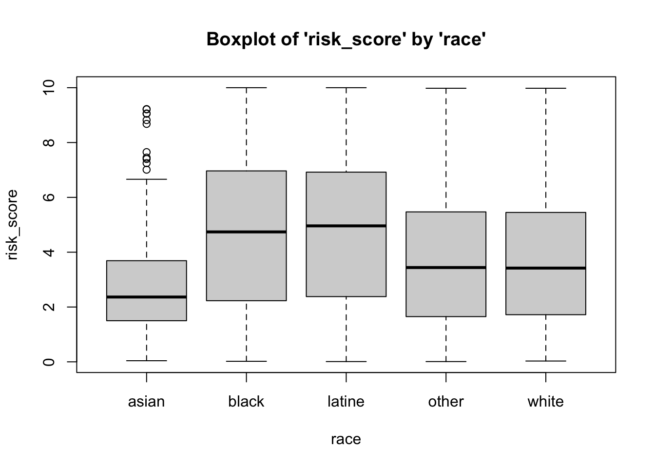
- We can see from the boxplots that the data
for all groups tend to be normally-distributed: All medians fall in the
center of the interquartile range. interquartile range is generally
centered between the whiskers. For
blackandlatinedefendants, the interquartile range is generally centered between the whiskers, whereas this range is lower forasian,other, andwhitedefendants. These data seem normal enough. It is safe to assume that these data are close enough to normal, since they aren’t drastically different from normal, and therefore safe to proceed with the statistical test.
4c. Normal Q-Q (Quantile-Quantile) Plots
The quantile-quantile plot is a visual tool to help us figure out if the empirical distribution of our variable fits (or rather, comes from) a theoretical normal distribution.
We assess normality an break this plot out by a grouping variable.

- We can see from the Q-Q plot that group
distributions of the outcome variable (
risk_score), the data are somewhat normal. However, it is important to notice that forblack,latine, andwhite(and, to some degree,asian) defendants, the data tend to curve away from the normality line at the tails of the distribution. This indicates some deviation from normality. Given that the data are normal enough, and there is no discernible pattern across the line (e.g. no strong curvilinear trend around normality line) for therisk_scorevariable for any group/level ofrace, it is safe to proceed with the statistical test.
- Across all three plots of
risk_scorebroken out byrace, the variables do not seem to drastically deviate from normality. Therefore,we can assume normality.
The One-Way ANOVA (F-Test) Calculation
The calculation for the F-Test is:
\(F = \frac{{MS}_{between}}{{MS}_{within}} = \frac{\frac{{SS}_{between}}{df_{between}}}{\frac{{SS}_{within}}{df_{within}}}\)
where…
- \({MS}_{between}\) is the mean
square for the treatment, effect, or between groups
- \({MS}_{within}\) is the mean
square for the error, or within groups
- \({SS}_{between} = \sum
n_{group}(\bar{X}_{group} - \bar{X}_{total})^2\) is the sum of
squares for the treatment, effect, or between groups; where \(\bar{X}_{total}\) is the grand mean, or the
mean of means
- \({SS}_{within} = \sum (X -
\bar{X}_{group})^2\) is the square for the error, or within
groups
In addition, the degrees of freedom (\(df\)) for the test is…
\(df_{between} = k - 1\); where \(k\) is the number of groups \(df_{within} = N - k\)
Running the One-Way ANOVA
To run the one-way ANOVA in R, we can use the ow.anova function from the
vannstats package.
For the One-Way ANOVA, within the ow.anova function, the data set
is listed first, followed by the dependent (interval-ratio level)
variable, and the independent (categorical) variable is listed
second.
Additionally, within the ow.anova function, you have the
option to request a means plot (by adding the call plot = T), and you also have the
option of requesting a Tukey’s HSD post-hoc comparisons test (by adding
the call hsd = T). I have
added both below
## Call:
## ow.anova(df = data1, var1 = risk_score, by1 = race, plot = T,
##     hsd = T)
##
## One-Way Analysis of Variance (ANOVA):
##                               df         SS         MS     F   p-value
## Between Groups (race)     4.0000   468.7904   117.1976 15.63 1.436e-12 ***
## Within Groups (race)   1733.0000 12994.7330     7.4984
## ---
## Signif. codes:  0 '***' 0.001 '**' 0.01 '*' 0.05 '.' 0.1 ' ' 1
##
## Tukey's HSD (Honestly Significant Difference):
##
##              Mean Difference        lwr     upr   p-value
## black-asian        1.6824844  0.7195372  2.6454 1.959e-05 ***
## latine-asian       1.6807265  0.7495067  2.6119 8.986e-06 ***
## other-asian        0.5524790 -1.0105918  2.1155    0.8708
## white-asian        0.6585677 -0.3135950  1.6307    0.3453
## latine-black      -0.0017579 -0.4455677  0.4421    1.0000
## other-black       -1.1300054 -2.4615410  0.2015    0.1398
## white-black       -1.0239167 -1.5482231 -0.4996 1.089e-06 ***
## other-latine      -1.1282475 -2.4370218  0.1805    0.1287
## white-latine      -1.0221588 -1.4856243 -0.5587 2.092e-08 ***
## white-other        0.1060887 -1.2321266  1.4443    0.9995
## ---
## Signif. codes:  0 '***' 0.001 '**' 0.01 '*' 0.05 '.' 0.1 ' ' 1
In the output above, we see the F-obtained value (15.63), the degrees of freedom between and within (4,1733), and the p-value (1.436e-12, or .000000000001436, which is much less than our set alpha level of .05).
To interpret the findings, we report the following information:
- The test used
- If you reject or fail to reject the null hypothesis
- The variables used in the analysis
- The degrees of freedom, calculated value of the test (\(F_{obtained}\)), and \(p-value\)
- \(F(df_{between},df_{within}) = F_{obtained}\), \(p-value\)
“Using a one-way ANOVA, I reject/fail to reject the null hypothesis that there is no mean difference between groups, in the population, \(F(?) = ?, p ? .05\)”
- “Using one-way ANOVA, I reject the null hypothesis that there is no mean difference in the risk scores assigned to defendants of different racial backgrounds, in the population, \(F(4,1733) = 15.63, p \lt .05\)”
Post-Hoc Checks: Which means differ?
After finding a significant result in your omnibus/overall F-test/ANOVA, to identify where the differences lie, you can do two things:
- Examine a means plot
- Run a Post-hoc significance test
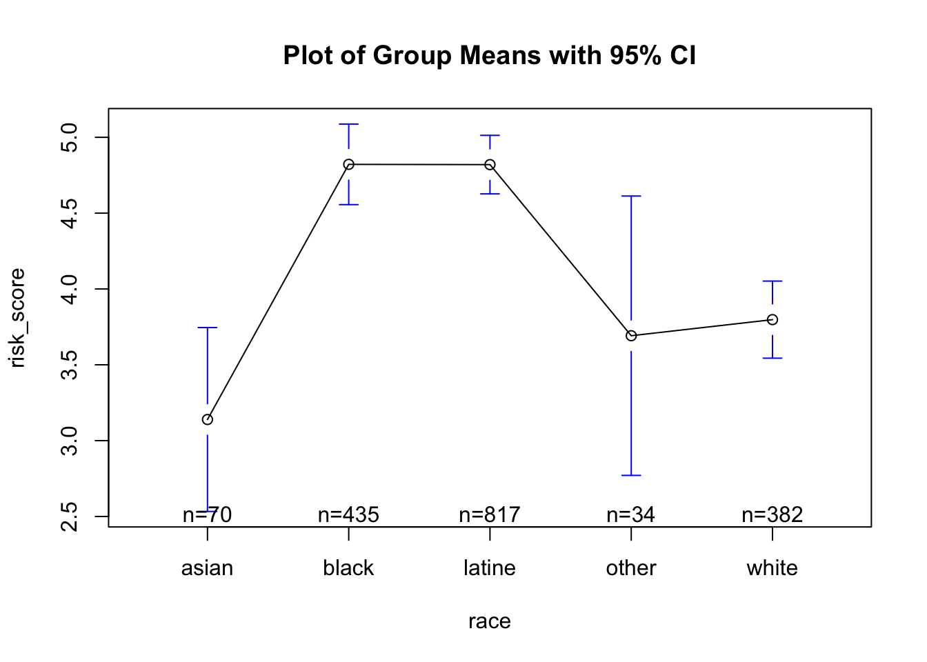
Means Plot
The means plot can be called from the ow.anova function. As seen
above:
- Here, we can see that it looks like
blackandlatinedefendants have extremely different (higher) mean risk scores than other racial categories (specifically,asianandwhitecategories) of defendants.
Post-Hoc Significance Test: Tukey’s HSD
And finally, we can see where the significantly different
mean comparisons are, with the Tukey’s HSD test… which can also be
called from the ow.anova
function. As seen above:
- Here, we see that risk scores for
blackdefendants are significantly different fromasiandefendants,latinedefendants are significantly different fromasiandefendants,whitedefendants are significantly different fromblackdefendants, and thatwhitedefendants are significantly different fromlatinedefendants.