One-Way ANOVA Example

Is there a mean difference in monthly income across different racial groups?

The Analysis of Variance (ANOVA)

The ANOVA is a bivariate (two variable) test that examines the differences in means between three or more groups, in effort to see if the differences reflect true differences that we could expect to find in the population. The resulting test calculates an F value.

For this example, the ANOVA works because we have have four groups (black, white, latinx, and other), and we’re examining each group’s mean monthly income to see if there is a true difference in income amongst racial groups in the population.

Load the Necessary Stuff

library(MASS)
library(psych)
library(vannstats)

Reading in the Data

ANOVA

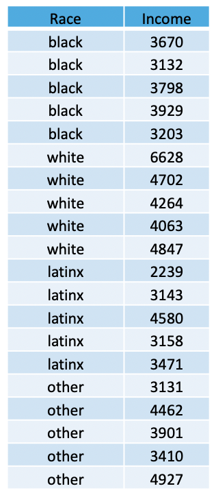
In the table (above), we have a total of 20 people, randomly-sampled. We see that we have a total of 5 people within each racial category (black, white, latinx, and other), and each individual has a monthly income value. We can use these data to create a data set, using a combination of the concatenate, c(), data frame data.frame, and the repeat rep() functions.

The repeat function comes in handy when you have to type out the same values over and over again. This function has two arguments: 1) the thing you want to repeat, and 2) the number of times you want to repeat it.

Using this logic, we can apply the repeat function to create each variable, concatenating across the various categories of each variable, and combine these variables into a data frame… as such…

race <- c(
  rep("black",5),
  rep("white",5),
  rep("latinx",5),
  rep("other",5))

inc <- c(3670, 3132, 3798, 3929, 3203, 6628, 4702, 4264, 4063, 4847, 2239, 3143, 4580, 3158, 3471, 3131, 4462, 3901, 3410, 4927)

Next, we merge the variables into one data frame, using the following:

data <- data.frame(race,inc)

Now we can call the data…

data

##      race  inc
## 1   black 3670
## 2   black 3132
## 3   black 3798
## 4   black 3929
## 5   black 3203
## 6   white 6628
## 7   white 4702
## 8   white 4264
## 9   white 4063
## 10  white 4847
## 11 latinx 2239
## 12 latinx 3143
## 13 latinx 4580
## 14 latinx 3158
## 15 latinx 3471
## 16  other 3131
## 17  other 4462
## 18  other 3901
## 19  other 3410
## 20  other 4927

Assumptions and Diagnostics for the ANOVA

The assumptions for an ANOVA are…

Independence of Observations
Equal Sample Sizes
Homogeneity of Variance
Normality

1. Independence of Observations (Examine Data Collection Strategy)

Groups are not related or dependent upon each other. Cases can’t be in more than one group. No ties between observations. Examine data collection strategy to see if there are linkages between observations.
- These data were randomly sampled. Therefore, we meet the assumption of independence of observations.

2. Equal Sample Sizes (Examine N for each group)

The number of cases in each group should be relatively similar.

3. Homogeneity of Variance (Examine SD² for each group)

All groups have approximately equal variances (SD²). The distributions (or spread) for the groups are approximately equal. Keppel & Zedeck (1989) suggest that variance comparison should not exceed 10:1 ratio (or… alternatively, the SDs, when compared, should not exceed around a 3:1 ratio). For both of the above assumptions, we can examine the univariate data table, broken out by group:

describeBy(data$inc, data$race)

## 
##  Descriptive statistics by group 
## group: black
##    vars n   mean     sd median trimmed    mad  min  max range  skew kurtosis     se
## X1    1 5 3546.4 358.68   3670  3546.4 383.99 3132 3929   797 -0.16    -2.17 160.41
## ------------------------------------------------------------------ 
## group: latinx
##    vars n   mean    sd median trimmed    mad  min  max range skew kurtosis    se
## X1    1 5 3318.2 842.1   3158  3318.2 464.05 2239 4580  2341 0.25    -1.45 376.6
## ------------------------------------------------------------------ 
## group: other
##    vars n   mean     sd median trimmed    mad  min  max range skew kurtosis     se
## X1    1 5 3966.2 738.26   3901  3966.2 831.74 3131 4927  1796 0.13    -1.99 330.16
## ------------------------------------------------------------------ 
## group: white
##    vars n   mean     sd median trimmed    mad  min  max range skew kurtosis     se
## X1    1 5 4900.8 1016.5   4702  4900.8 649.38 4063 6628  2565 0.82    -1.21 454.59

The sample size for each group is exactly the same for all groups. Therefore, we have met the assumtption for equal sample sizes. We can also see that, when comparing the SD for all groups, there is not a ratio larger than 3:1. For these data, the largest discrepancy between SDs for each group is between black individuals (SD = 358.68) and white individuals (SD = 1016.5), which is less than the 3:1 ratio suggested. Therefore, we have met the assumption for homogeneity of variance.

4. Normality (Examine Plots: Histogram, Q-Q Normality Plots, Box-and-Whiskers Plots)

Distribution must be relatively normal.

4a. Histogram

Plot the histogram for Monthly Income (Y variable) broken out by Racial Category (levels of the X variable), overlaying a normal curve…

hst(data, inc, race)

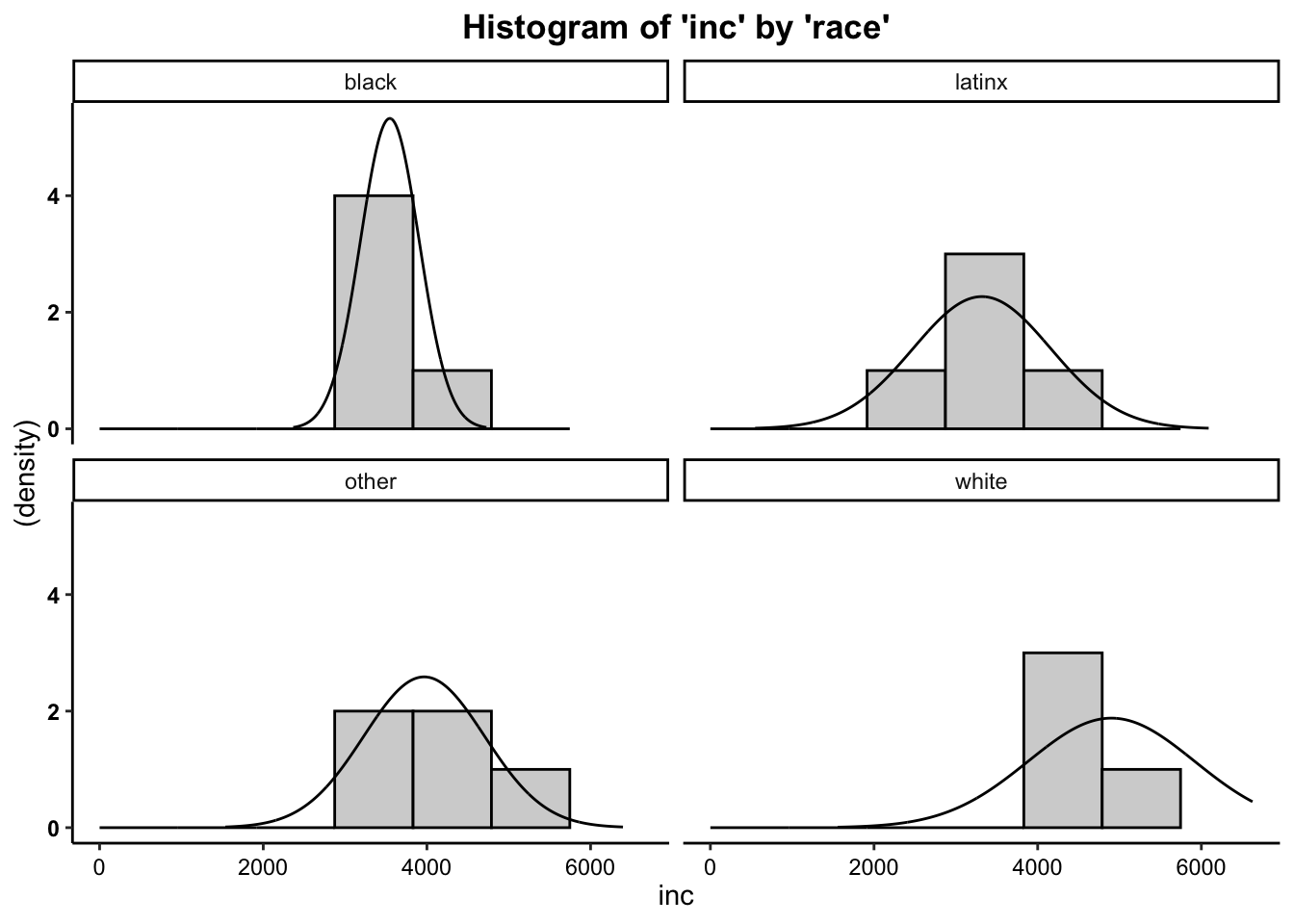
We can see from the histogram that for group distributions of the outcome variable (beers), the data are moderately positively skewed (with the exception of the distribution of scores for black individuals). Although these are moderately skewed, it is safe to assume that these data are close enough to normal to proceed with the statistical test.

4b. Boxplots (Box-and-Whisker Plots)

Boxplots also provide a visual representation of the normality of a distribution. The boxplot has a box, a line through the box, two whiskers on either end of the box, and sometimes dots/points outside the whiskers. Below, we get a sense of what each part of the boxplot represents…

Bottom (or left end) of the whisker represents the minimum score for that variable’s distribution
Bottom (or left end) of the box represents the first quartile (the 25th percentile case)
Middle line (or dot) inside the box represents the median, also known as the second quartile (the 50th percentile case)
Top (or right end) of the box represents the third quartile (the 75th percentile case)
Top (or right end) of the whisker represents the maximum score for that variable’s distribution
Outside dots represent outliers - extreme high or extreme low values for that variable.

To tell if a variable is normally-distrubted using the box-and-whisker plot, generally, we want to see that there is some distance between the box and the end of the whiskers, that the box isn’t pushed too close to either whisker, that the median line (dot) is near the center of the box, and that there aren’t many outliers (dots) on the outside of the whiskers.

To plot a boxplot of Monthly Income, broken out by Race, we can do the following…

box(data, inc, race)

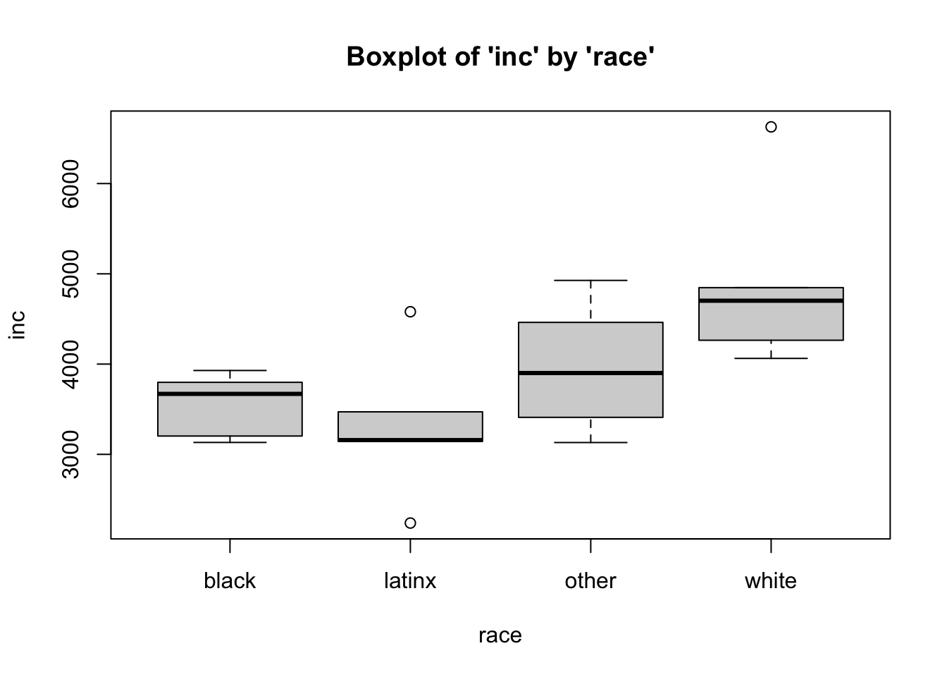
We can see from the boxplots that for the black and other groups are somewhat normally distributed. The data for latinx and white individuals, however, possesses some outliers, and the median falls near or on the edge of the interquartile range. In addition, the minimum and maximum scores are missing for latinx individuals while the maximum is missing for white individuals (rather, those scores are read as extremes or outliers). These plots may give us some pause in proceeding. In many cases, finding distributions like this would warrant further data collection (e.g. there may be too few cases in this sample, which is why many are perceived as outliers). However, for this example, the data seem normal enough. It is safe to assume that these data are close enough to normal, since they aren’t drastically different from normal, and therefore safe to proceed with the statistical test.

4c. Normal Q-Q (Quantile-Quantile) Plots

The quantile-quantile plot is a visual tool to help us figure out if the empirical distribution of our variable fits (or rather, comes from) a theoretical normal distribution.

We assess normality an break this plot out by a grouping variable.

qq(data, inc, race)

We can see from the Q-Q plot that for group distributions of the outcome variable (monthly income), the data are somewhat normal, since there is no discernible pattern across the line (e.g. no strong curvilinear trend around normality line) for the income variable for any group/level (race). It is therefore safe to proceed with the statistical test.
Based on the the three visual depictions above, the data seem normally-distributed. Therefore, we meet the assumption of normality.

The One-Way ANOVA (F-Test) Calculation

The calculation for the F-Test is:

\(F = \frac{{MS}_{between}}{{MS}_{within}} = \frac{\frac{{SS}_{between}}{df_{between}}}{\frac{{SS}_{within}}{df_{within}}}\)

where…

\({MS}_{between}\) is the mean square for the treatment, effect, or between groups
\({MS}_{within}\) is the mean square for the error, or within groups
\({SS}_{between} = \sum n_{group}(\bar{X}_{group} - \bar{X}_{total})^2\) is the sum of squares for the treatment, effect, or between groups; where \(\bar{X}_{total}\) is the grand mean, or the mean of means
\({SS}_{within} = \sum (X - \bar{X}_{group})^2\) is the square for the error, or within groups

In addition, the degrees of freedom (\(df\)) for the test is…
\(df_{between} = k - 1\); where \(k\) is the number of groups \(df_{within} = N - k\)

Running the One-Way ANOVA in R

To run the one-way ANOVA in R, we take the summary (output) of the analysis of variance aov function.

For the ANOVA, within the aov function, the dependent (interval-ratio level) variable is listed first and the independent (discrete/categorical) variable is listed second, separated by a tilde ~.

ow <- ow.anova(data, inc, race, plot = T, hsd = T)

summary(ow)

## Call:
## ow.anova(df = data, var1 = inc, by1 = race, plot = T, hsd = T)
## 
## One-Way Analysis of Variance (ANOVA): 
##                            df      SS      MS      F p-value  
## Between Groups (race)       3 7325888 2441963 4.0429 0.02569 *
## Within Groups (race)       16 9664314  604020                 
## ---
## Signif. codes:  0 '***' 0.001 '**' 0.01 '*' 0.05 '.' 0.1 ' ' 1
## 
## Tukey's HSD (Honestly Significant Difference): 
## 
##              Mean Difference       lwr    upr p-value  
## latinx-black        -228.200 -1634.495 1178.1 0.96579  
## other-black          419.800  -986.495 1826.1 0.82793  
## white-black         1354.400   -51.895 2760.7 0.06113 .
## other-latinx         648.000  -758.295 2054.3 0.56513  
## white-latinx        1582.600   176.305 2988.9 0.02480 *
## white-other          934.600  -471.695 2340.9 0.26628  
## ---
## Signif. codes:  0 '***' 0.001 '**' 0.01 '*' 0.05 '.' 0.1 ' ' 1

In the output above, we see the F-obtained value (4.043), the degrees of freedom between and within (3,16), and the p-value (.0257, which is less than our set alpha level of .05).

To interpret the findings, we report the following information:

The test used
If you reject or fail to reject the null hypothesis
The variables used in the analysis
The degrees of freedom, calculated value of the test (\(F_{obtained}\)), and \(p-value\)
- \(F(df_{between},df_{within}) = F_{obtained}\), \(p-value\)

“Using a one-way ANOVA, I reject/fail to reject the null hypothesis that there is no mean difference between groups, in the population, \(F(?) = ?, p ? .05\)”

“Using one-way ANOVA, I reject the null hypothesis that there is no mean difference between the monthly income of different racial categories, in the population, \(F(3,16) = 4.043, p \lt .05\)”

Post-Hoc Checks: Which means differ?

After finding a significant result in your omnibus/overall F-test/ANOVA, to identify where the differences lie, you can do two things:

Examine a means plot
Run a Post-hoc significance test

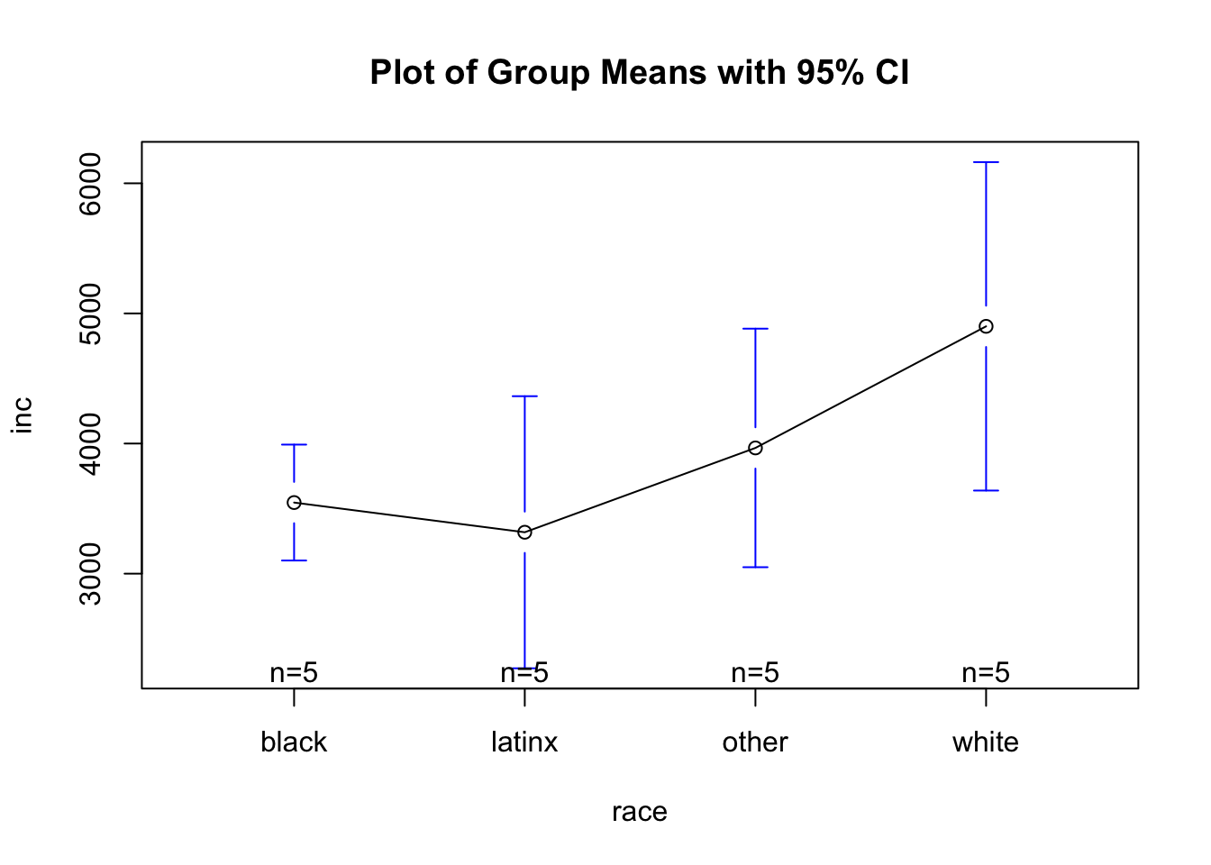
Means Plot

As seen in the plot above:

Here, we can see that it looks like whites have higher monthly incomes than others. Yet to see, statistically, if group means differ, we have to run post-hoc tests that compare all possible pairs of means to determine which differences are statistically significant.

Post-Hoc Significance Test: Tukey’s HSD

As seen in the output above:

Here, we see that the only significant difference lies between white’s mean monthly income and latinx’ mean monthly income.