Getting Started with RStudio
What is RStudio?
RStudio is a program that wraps around R, such that, when you open it, it will run R in the background. RStudio is an IDE (Integrated Development Environment) with a graphical user interface that allows you to “see” what you’re doing (e.g. point-and-click gestures).
The RStudio Development Environment
Open the RStudio program, which should be linked to R.
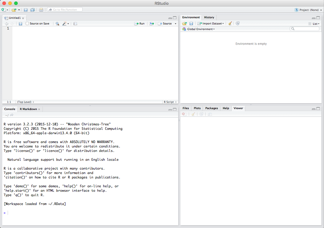
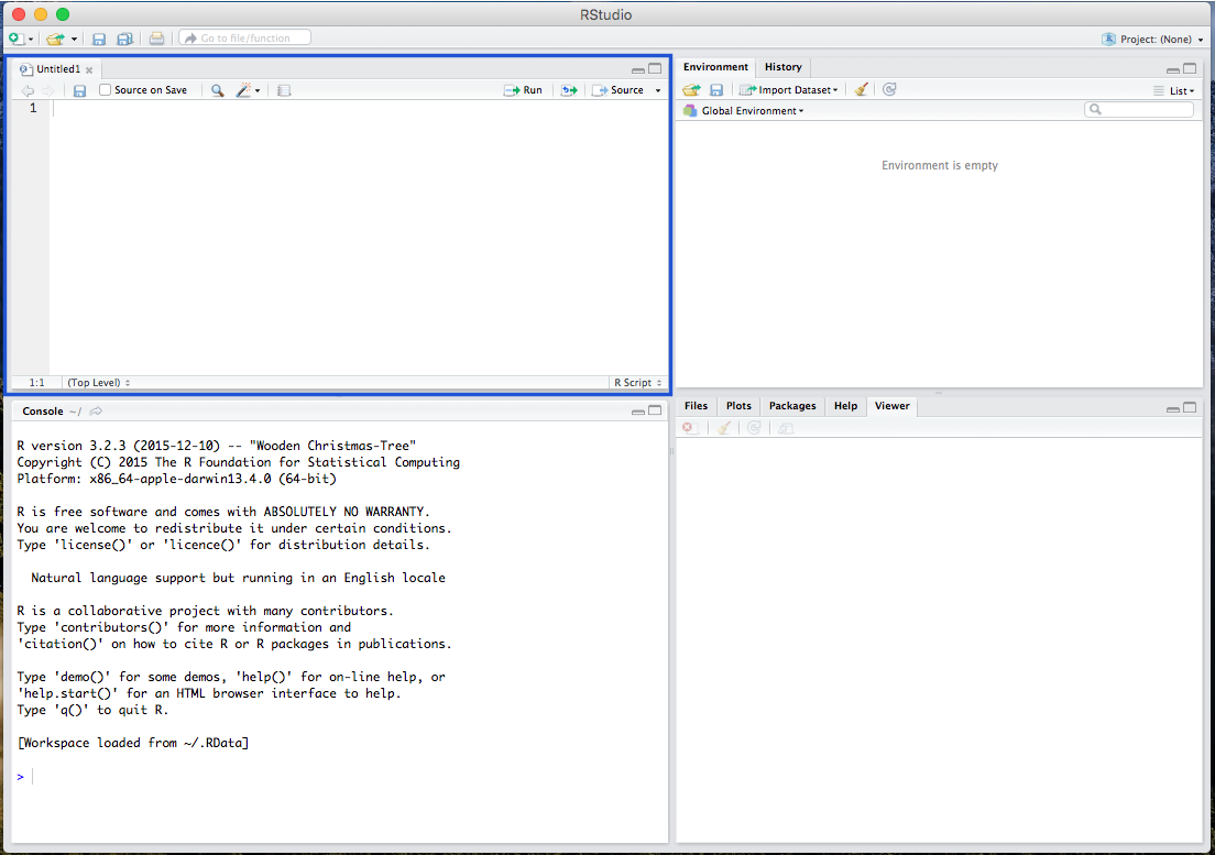
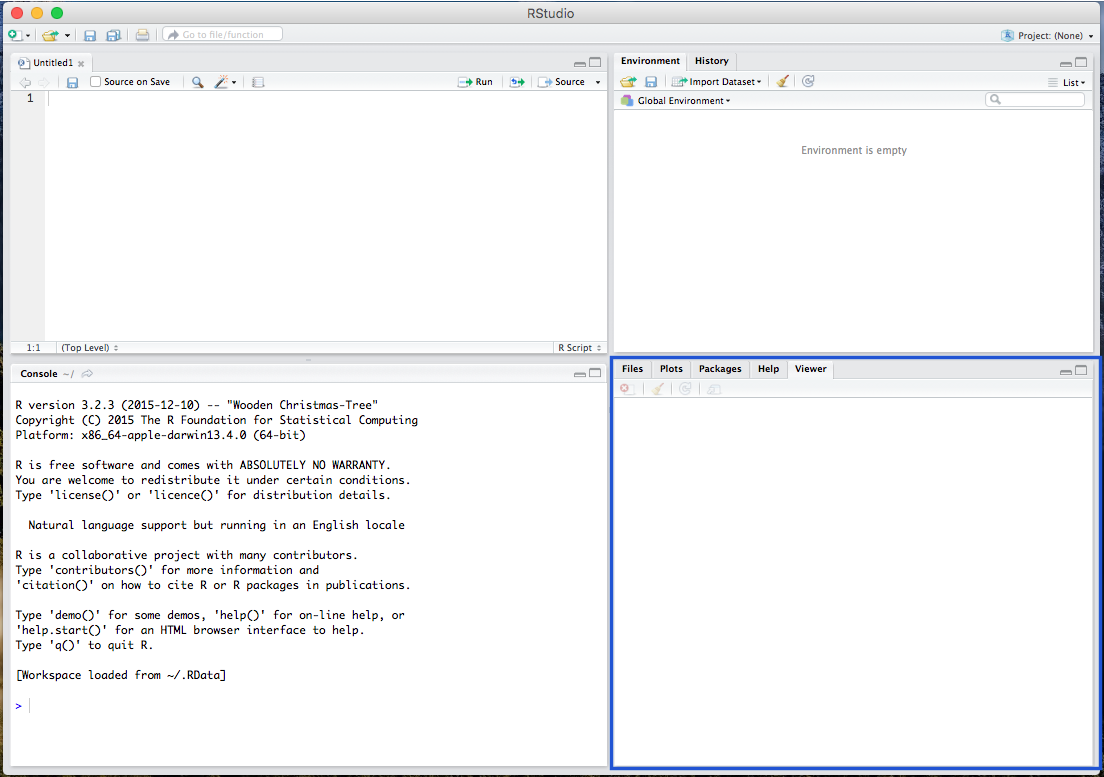
There are various windows within RStudio. The first is the Script window, where all your codes are viewable:
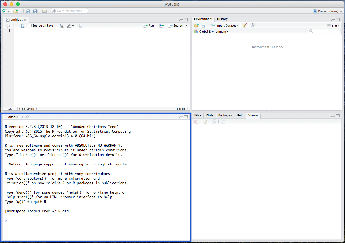
The Console window where you paste and run your code (which is where R is directly run):
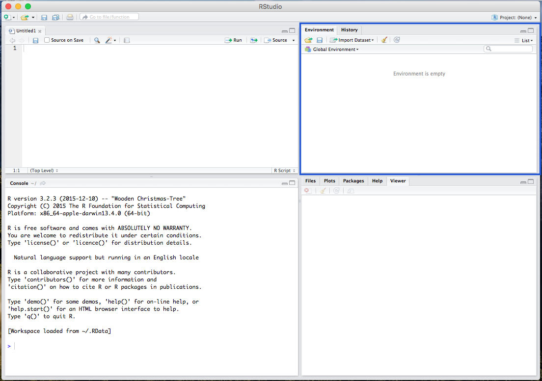
The Environment window, where your data and background processes are viewable:
And the Plot/Viewer window, where your output figures/diagrams, help information, and file viewer are located:
Getting Familiar with R
Calculations
In R/RStudio, we can use the Script (and Console) window to make calculations. For example, we can run the following…
## [1] 5The Assignment Operator: Creating Objects
The great thing about R is that, because it is an object-oriented
programming language, you can assign object names to
any calculation or data set. This creates a working copy of the
calculation (or data set) in R’s memory that you can run operations on.
To do so, you simply must assign an object name using a left
arrow (the assignment operator) like this: new_object <- dataset. For
example, we could run…
… and then run…
## [1] 5… which gives us the same result, but now we can run manipulations on
the new object (or variable) x:
## [1] 2.5Removing Objects from your Environment
Many times, we’ll be working with several objects, and ultimately
decide that some of them are no longer needed. In this case, we would
want to tidy up our environment by removing an object. To do so, we must
use the rm function. You
can do it like this, changing the word “OBJECT” to the name of the
object that you’re trying to remove from the R environment: rm(OBJECT).
Commenting
Througout any script, you’ll also notice a line of text with a pound
sign (e.g. hashtag) preceding it, like this #this is a how to calculate a mean.
This is a comment, which is just a note to yourself.
Comments remind the user what the a bit of code is supposed to do.
Packages and Libraries
Installing Packages
Because R is and open-source statistical program, many of its
functions are built by programmers in the form of
packages. Most of these are published and hosted on the
Comprehensive R Archive Network
(CRAN) website. We will be using 3 main packages in this exercise:
the MASS, the psych, and the
vannstats package.
Install the packages from the repository (copy and paste the lines below)
Once you’ve successfully installed the packages, a small version of them will exist on your computer. This means you will not have to reinstall the package, unless the package is 1) updated, and 2) you require the additional functionality included in the updated version.
Importantly, these packages will be hidden in the background, and will not be loaded until you tell R to load them for use.
Working with Stock Data Sets in R
Fortunately, nearly every package in R comes with a data set that R
users can use. To see which stock data sets are installed in your
version of R, use the data() function. The
MASS package, for example,
comes with a great data set on car manufacturers called mtcars.
Getting Information about/Codebook for Stock Data Sets in R
Before loading the data set, you might want to know more about it. In
order to get information about a data set (including the data set
description, the size of the data set, and variable names and
descriptions), you need to ask R. To do so, you need use the
??
(double-question-mark) function as such…
Using Stock Data Sets in R
To use the mtcars data
set, you must call it. Calling the data will load it into your console
window. To call a stock data set, just type in the name of the data set
(Note: The data set you’re calling must come from a package that is
already LOADED into your R session). Because the MASS package is
already loaded, we can call our mtcars data set
as such…
##                      mpg cyl  disp  hp drat    wt  qsec vs am gear carb
## Mazda RX4           21.0   6 160.0 110 3.90 2.620 16.46  0  1    4    4
## Mazda RX4 Wag       21.0   6 160.0 110 3.90 2.875 17.02  0  1    4    4
## Datsun 710          22.8   4 108.0  93 3.85 2.320 18.61  1  1    4    1
## Hornet 4 Drive      21.4   6 258.0 110 3.08 3.215 19.44  1  0    3    1
## Hornet Sportabout   18.7   8 360.0 175 3.15 3.440 17.02  0  0    3    2
## Valiant             18.1   6 225.0 105 2.76 3.460 20.22  1  0    3    1
## Duster 360          14.3   8 360.0 245 3.21 3.570 15.84  0  0    3    4
## Merc 240D           24.4   4 146.7  62 3.69 3.190 20.00  1  0    4    2
## Merc 230            22.8   4 140.8  95 3.92 3.150 22.90  1  0    4    2
## Merc 280            19.2   6 167.6 123 3.92 3.440 18.30  1  0    4    4
## Merc 280C           17.8   6 167.6 123 3.92 3.440 18.90  1  0    4    4
## Merc 450SE          16.4   8 275.8 180 3.07 4.070 17.40  0  0    3    3
## Merc 450SL          17.3   8 275.8 180 3.07 3.730 17.60  0  0    3    3
## Merc 450SLC         15.2   8 275.8 180 3.07 3.780 18.00  0  0    3    3
## Cadillac Fleetwood  10.4   8 472.0 205 2.93 5.250 17.98  0  0    3    4
## Lincoln Continental 10.4   8 460.0 215 3.00 5.424 17.82  0  0    3    4
## Chrysler Imperial   14.7   8 440.0 230 3.23 5.345 17.42  0  0    3    4
## Fiat 128            32.4   4  78.7  66 4.08 2.200 19.47  1  1    4    1
## Honda Civic         30.4   4  75.7  52 4.93 1.615 18.52  1  1    4    2
## Toyota Corolla      33.9   4  71.1  65 4.22 1.835 19.90  1  1    4    1
## Toyota Corona       21.5   4 120.1  97 3.70 2.465 20.01  1  0    3    1
## Dodge Challenger    15.5   8 318.0 150 2.76 3.520 16.87  0  0    3    2
## AMC Javelin         15.2   8 304.0 150 3.15 3.435 17.30  0  0    3    2
## Camaro Z28          13.3   8 350.0 245 3.73 3.840 15.41  0  0    3    4
## Pontiac Firebird    19.2   8 400.0 175 3.08 3.845 17.05  0  0    3    2
## Fiat X1-9           27.3   4  79.0  66 4.08 1.935 18.90  1  1    4    1
## Porsche 914-2       26.0   4 120.3  91 4.43 2.140 16.70  0  1    5    2
## Lotus Europa        30.4   4  95.1 113 3.77 1.513 16.90  1  1    5    2
## Ford Pantera L      15.8   8 351.0 264 4.22 3.170 14.50  0  1    5    4
## Ferrari Dino        19.7   6 145.0 175 3.62 2.770 15.50  0  1    5    6
## Maserati Bora       15.0   8 301.0 335 3.54 3.570 14.60  0  1    5    8
## Volvo 142E          21.4   4 121.0 109 4.11 2.780 18.60  1  1    4    2
While this is great, and the data set is loaded into your console
window, you will need a local copy to run operations on. To create a
local copy (an object) so that you can run manipulations on the mtcars data, you should create a
new object, like this:
Like above, you can now call data1, and it will load the same
data set into your console window (not shown here). In addition, in
RStudio, after you give the data a new name (converting it to a usable
object), you can view the data in your upper-right
Environment window.
Calling Variable Information
To call a specific variable or column within the data set,
you simply use the dollar sign operator $, in the form of data$variable. To call the mpg variable from the new data1 data set, we use the
following.
##  [1] 21.0 21.0 22.8 21.4 18.7 18.1 14.3 24.4 22.8 19.2 17.8 16.4 17.3 15.2 10.4
## [16] 10.4 14.7 32.4 30.4 33.9 21.5 15.5 15.2 13.3 19.2 27.3 26.0 30.4 15.8 19.7
## [31] 15.0 21.4
Additional R Resources
R for Data Science
Dr. Matt
Blackwell’s Advanced Quant Methods Course in Political Science
Dr. Chris Bail’s Data &
Society Course
Summer Institute in Computational Social Science
- [ Github
Repo of 2020 Materials, 2019 Materials, 2020
Videos (with Links) ]