Reading-in Data
Directories
A directory is simply a folder on your computer. This is where your files are located. However, you must tell R to “look” into this folder to read/write files to it. This is called setting your working directory.
Setting the Working Directory
Before running analyses, you have to set your working directory. This is the folder where your data/output are and will be saved. For example, I use the following:
This will be different for you. To set your working directory, use
setwd("directory"), and
replace the word “directory” with the pathname of the folder
you want to be your directory (or under the Session
menu, select Set Working Directory, then select
Choose Directory and navigate to your desired
folder).
Reading in CSV Data
Local Files: Reading in a CSV Data Set from your Own Computer
Many data sets that researchers work with come in the form of a CSV file. A CSV (Comma Separated Values) file is just a Microsoft Excel spreadsheet (with rows as observations and columns as variables), that is converted into CSV format.
A CSV file must be “read” into the R environment for you to use it.
To do so, you’ll have to call in the CSV file (data set) with one of R’s
functions: the read.csv
function. Additionally, you will have to give the CSV a new object name
(using the assignment operator <-), so we can place
it in our working environment. You can do it like this, changing the
word Pathname/to/CSV/file.csv to the pathname to the csv
file you’re reading into the R environment: data1 <- read.csv("Pathname/to/CSV/file.csv", header=TRUE, sep=",").
The pathname to a file is the digital address to a file on your
current (local) machine. Here, to our file called file.csv
is "Pathname/to/CSV/file.csv"
Some important things about the pathname … which is obviously basic computer stuff: 1) every item on your computer has an address/pathname, 2) the pathnames are unique to YOUR computer (e.g. the structure of files/directories on your computer, so you can’t just copy and paste it to use on another computer, since the other computer will likely have a different setup/structure/set of files and directories), and 3) the pathname changes every time you move your file to a new directory.
To get the pathname to a file, you should right-click on it. Within
this menu, on a Mac, simply 1) hold down the option key, and select
copy "file.csv" as Pathname, then 2) then replace the
"Pathname/to/CSV/file.csv" with the Pathname to your file
by pasting the copied Pathname. To see this in action, watch the next
few minutes of
this
video I created a few years ago.
For example, let’s assume I have saved the mtcars data
as cars.csv in my PA606 folder/directory on my Desktop. I
would find it, right click on it, and copy the pathname to the file
below, reading in the data set as an object call data1:
Online Files: Reading in a CSV Data Set from a URL
Sometimes you’ll want to use a CSV file from a website, where you
have a direct link to the CSV. For example, I uploaded the same
mtcars data set as cars.csv on my
website.
To read in this data set, you can either download/save it on your own
machine, then use the steps above (reading in a CSV from your own
computer), or you can read it directly into R using the
RCurl package. This means that first, you’ll have to,
first, install the RCurl package, then load the package,
and use this code to read in the linked CSV as a new object called
data1: data1 <- read.csv(text=getURL("URL-to-CSV.csv")).
Within the quotations, replace URL-to-CSV.csv with the
actual URL link to the CSV file, as seen here:
install.packages("RCurl")
library(RCurl)
data1 <- read.csv(text=getURL("www.burrelvannjr.com/cars.csv"))
data1
Reading in RData Files
Local Files: Reading in an RData Data Set from your Own Computer
R also has it’s own native data formats that retain many of the
chraracteristics of the data set (so they don’t get lost upon saving in
different formats). These are known as RData files
(saved as .RData' or.Rda’).
The RData file must be “read” (or rather, loaded) into the R
environment using the load function, as such:
data1 <- load("Pathname/to/CSV/file.RData")
For example, let’s assume I have saved the mtcars data
as cars.RData in my PA606 folder/directory on my Desktop. I
would find it, right click on it, and copy the pathname to the file
below, reading in the data set as an object call data1:
Reading in Google Sheets Data
Online Files: Reading in a Google Sheet
In a more complicated way, you can also access a GoogleSheet data
set. To do so, however, you need to authorize the
googlesheets4 package (within tidyverse package
family) API to essentially “speak to” Google Sheets… which means you
need to grant it access to a Google Sheet that YOU OWN.
This means that you need to respond to the package when it asks you to
grant access to your Google Drive account.
Because I can’t authorize it here (because it will open up a new
window and ask for credentials), I only provide you with the package to
install and load script… and have commented out the
read_sheet function that enables you to read in a Google
Sheet.
If you were to do this for yourself, you would: 1) remove the #, so
the line is no longer commented out, and 2) replace
URL-to-Google-Sheet with the actual URL link to the Google
Sheet you’re trying to read in.
install.packages("googlesheets4")
library(googlesheets4)
#data1 <- read_sheet("URL-to-Google-Sheet")
Generating New Data
Creating a List as an Object
Sometimes, for quick analyses, you may need to read in a list of
numbers (in your working Environment). To read in a list, you use the
concatenate c function. You
can create a list by replacing the word “LIST” from this with the actual
list: c(LIST).
To create an object out of a list of numbers, we could do the following…
Now that list is a
useable object, we can run manipulations and univariate statistics on it
(described below).
In addition, you can use the c or concatenate function to
manually input columns of data (variables) and merge
them into one data frame.
Let’s say someone sent you the following image:
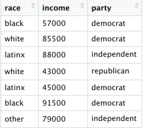
We could insert the data, one variable at a time, each as a new list object:
race <- c("black","white","latinx","white","latinx","black","other")
income <- c(57000,85500,88000,43000,45000,91500,79000)
party <- c("democrat","democrat","independent","republican","democrat","democrat","independent")
Next, we can view the lists by calling the object names:
## [1] "black" "white" "latinx" "white" "latinx" "black" "other"## [1] 57000 85500 88000 43000 45000 91500 79000## [1] "democrat" "democrat" "independent" "republican" "democrat"
## [6] "democrat" "independent"To merge these objects together, we use the cbind (or column bind) function –
which converts the list into a column (variable).
Converting an Object to a Data Frame
However, the best or more appropriate way is to merge objects into a
data frame, using the data.frame function.
And the data should now be presented as a data frame:
##     race income       party
## 1  black  57000    democrat
## 2  white  85500    democrat
## 3 latinx  88000 independent
## 4  white  43000  republican
## 5 latinx  45000    democrat
## 6  black  91500    democrat
## 7  other  79000 independent
Writing/Saving your Data as a Local File
You can save or write your data to a local file in several ways. For example, you can either write it as a CSV file, or save it as an RData file.
Writing Data as a Local CSV
To save your data as a CSV, you would use the write.csv
function, as such: